
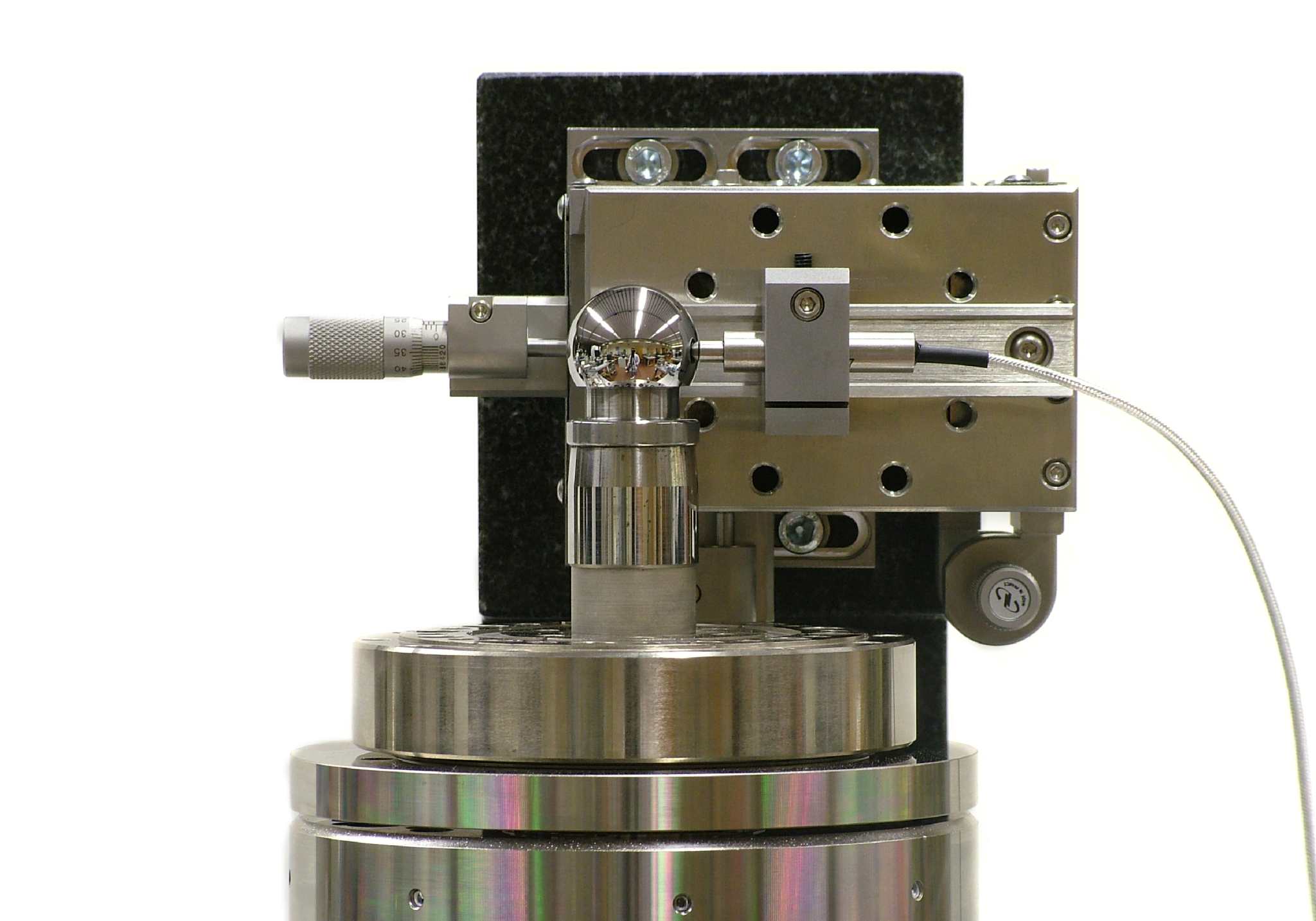
Thermal Drift in Precision Machines: How a Millikelvin Becomes a Nanometre
In a precision machine, temperature is a dimension. A positioning stage that is accurate to a few nanometres on the day it is qualified can lose that accuracy by lunchtime because the room warmed up, a motor dissipated a little more power, or an operator opened a door. The mechanics did not change. The temperature did, and every material in the machine responded to it.
This article walks through the engineering behind that effect: how small temperature changes turn into displacement, why the problem is dominated by time constants rather than by steady-state values, and how a combination of modelling and design keeps thermal error inside the error budget.
From temperature to displacement
To first order, a body of length L that changes temperature by ΔT changes length by
ΔL = α · L · ΔT
where α is the coefficient of thermal expansion (CTE). The numbers look harmless until they are compared with the accuracy of the machine. The table shows the drift of a 200 mm structural element for a temperature change of one millikelvin.
| Material | CTE (10⁻⁶ per K) | Drift for 200 mm at 1 mK |
|---|---|---|
| Aluminium 6061 | about 23 | about 4.6 nm |
| Structural steel | about 12 | about 2.4 nm |
| Invar 36 | about 1.3 | about 0.26 nm |
| Zerodur | about 0.02 | about 0.004 nm |
A single millikelvin on a 200 mm aluminium part is already about 4.6 nm. A realistic disturbance of 0.5 K is 2.3 µm, three orders of magnitude above the nanometre-level targets common in semiconductor and metrology equipment. Low-expansion materials such as Invar and Zerodur reduce the sensitivity, but they bring their own trade-offs in stiffness, mass, cost, maintainability and long-term dimensional stability. In practice, material choice is only the first lever.
Drift is a transient problem
Most thermal errors are not caused by a machine being warm. They are caused by a machine that is still changing temperature. The simplest useful description is a lumped-parameter model of a body with thermal capacity C, coupled to its surroundings through a thermal resistance R, and heated by a power P:
C · dT/dt = P − (T − T_amb) / R, τ = R · C
Take a 2 kg aluminium block (specific heat about 900 J/kgK, so C is about 1800 J/K) that exchanges heat with the air through natural convection. With h of about 10 W/m²K over 0.1 m², the coupling is 1 W/K. The time constant is then about 1800 s, or 30 minutes. Two consequences follow directly.
Small powers matter. A constant 0.5 W dissipated in the block eventually raises it by P · R = 0.5 K. That is the 2.3 µm from the table, produced by a power smaller than a single LED indicator.
The block acts as a low-pass filter. For an ambient fluctuation with angular frequency ω, the temperature of the block follows with an amplitude ratio of 1/√(1 + (ωτ)²). A one-hour cycle, for example from air conditioning, is attenuated to about 30 percent. A 24-hour cycle passes almost untouched, at about 99 percent. Thermal mass therefore protects against fast disturbances and does nothing against slow ones, which is why long-term stability specifications such as a few millikelvin per hour are so demanding.
Choosing the right model for the question
Lumped models are excellent for understanding which time constants and heat paths dominate. They cannot tell you where a gradient builds up inside a complex structure, how a bracket bends when one side warms faster than the other, or how a real contact interface behaves. That is where finite element analysis comes in. In our work on thermal modelling and simulation services, we typically use FEM to resolve the spatial temperature field and the resulting deformation, then reduce the result to a compact model that can run in the time domain, next to the control system and the other physical domains of the machine. The same compact model can later be fed with measurement data and used as a digital twin.
The physics behind these models, conduction, convection and radiation, is summarised in our overview of heat transfer fundamentals for engineering systems. The practical point is that each mechanism has a different sensitivity to the design: convection coefficients depend on airflow, radiation on surface emissivity, and conduction on the geometry and the quality of every joint in the path.
Design strategies that keep drift inside the budget
Once the dominant heat paths are known, thermal behaviour can be designed rather than corrected. In precision machine design, the following measures are used in combination:
- Reduce and relocate heat sources. Motors, amplifiers and sensors are placed away from the measurement loop, and their power is minimised or duty-cycled.
- Separate the metrology frame from the force frame, so that heat entering the structure that carries the loads does not reach the structure that defines the position.
- Use symmetry and a defined thermal centre. A symmetric design expands about a known point, which turns an unpredictable error into a repeatable one that can be calibrated or ignored.
- Match materials where they are joined, and use compliant or kinematic mounts so that residual differences in expansion do not turn into stress and distortion.
- Stabilise the environment actively where passive measures are not enough, for example with temperature-controlled water loops and shrouds, with the control loop designed alongside the thermal model.
Validating the result
A thermal design is only trustworthy when the model has been compared with measurements at the level of stability that matters. For a semiconductor application, we designed a thermal validation tool for semiconductor equipment around a stability target of a few millikelvin per hour. Using the numbers above, even 1 mK per hour on a 200 mm aluminium part is about 4.6 nm per hour, which shows why the target had to be treated as a design requirement from the first concept rather than as a test result at the end.
Closing the loop between model and hardware is the purpose of prototype build and test services: the prototype is instrumented, the measured time constants are compared with the predicted ones, and the model is corrected before the design is frozen.
Key takeaways
Thermal drift is controlled by three things: how much heat enters the machine, how quickly the structure responds, and how much the structure expands for each kelvin. A good design addresses all three, and a good model tells you which one dominates before any hardware is built. If thermal stability is limiting the performance of your machine or instrument, you can talk to our precision engineering team about your requirements.